Fourier pricing
An option price is a discounted average of its future payoff under the risk-neutral distribution. Fourier pricing evaluates that average using the distribution's characteristic function.
A different view of the same distribution
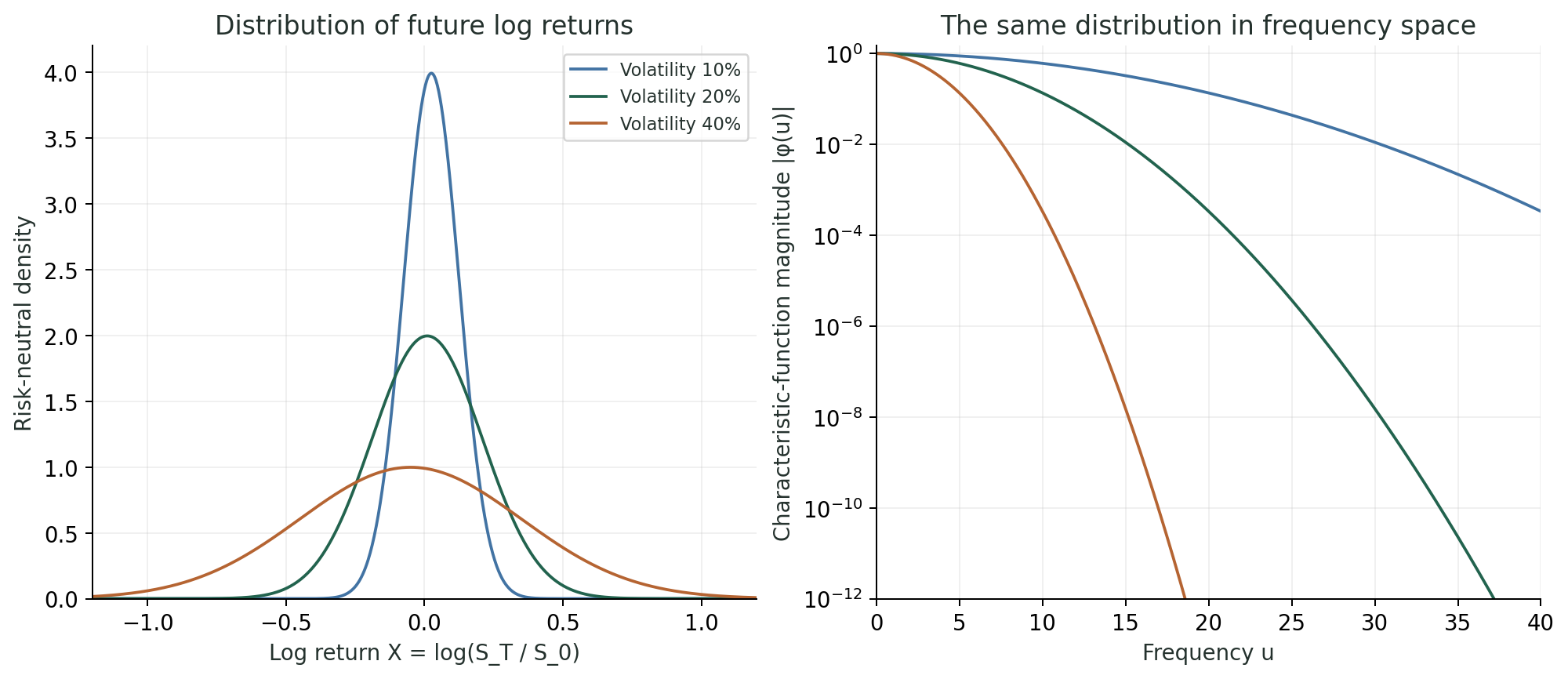
For the log return \(X=\log(S_T/S_0)\), the characteristic function is
\[ \phi(u)=\mathbb E^{\mathbb Q}[e^{\mathrm{i}uX}]. \]It describes the distribution through its response to waves of different frequencies. In Black–Scholes, log returns are Gaussian: a broader distribution has a faster-decaying frequency spectrum.
Recover the price
The characteristic function carries the model information. A known weight accounts for the call payoff. Combine them and integrate in frequency space to recover the price, using damping to make the transform well defined.
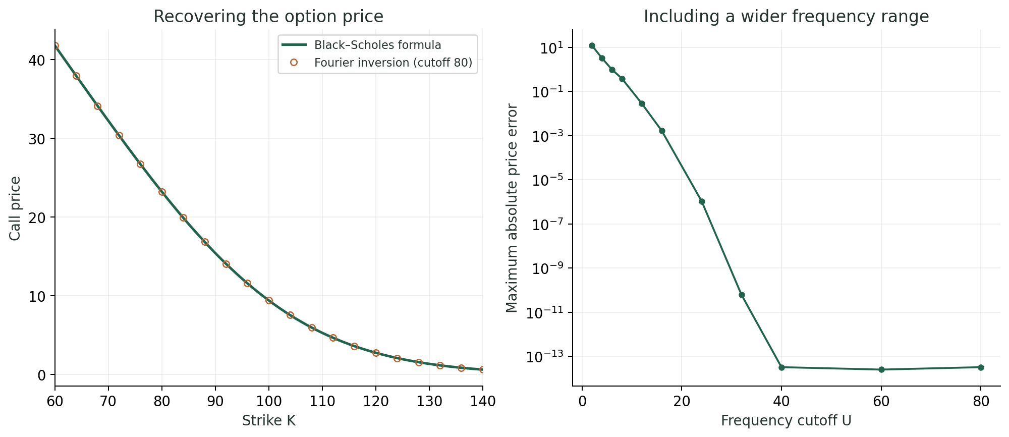
Black–Scholes gives us an exact reference. Fourier methods are also useful for models with a tractable characteristic function but no simple option-pricing formula.
Where compression comes in
Fourier pricing supplies an integral to compute. Low-rank methods can exploit additional structure in that integrand or its parameter dependence. The price-surface note illustrates what low rank and low polynomial degree look like in a simple example.
Methods, formula, and reproducibility
We use the Carr–Madan damped Fourier formula, with log strike k = log(K/S₀) and the characteristic function of X = log(S_T/S₀). The transformed quantity is the normalized call price multiplied by exp(αk), with α = 1.5. The integrand uses the characteristic function at the shifted argument u − i(α + 1). After inversion we remove the damping and multiply by S₀.
The computation uses adaptive quadrature over 0 ≤ u ≤ U, with absolute and relative integration tolerances of 10⁻¹². It does not use an FFT. The convergence plot shows the maximum absolute price error over the 81 tested strikes. At large cutoffs, numerical roundoff dominates. Frequency decay and the required cutoff depend on the model and parameters; this example does not establish a speedup or a low-rank bound.
The code checks the characteristic function against direct integration of the density, verifies its normalization and risk-neutral first moment, and compares prices across several strikes, volatilities, maturities, and damping choices with the Black–Scholes formula.
Reproduction code · Prices and convergence data. Keep bs1d_demo.py beside the reproduction script.
Related research: Learning parameter dependence for Fourier-based option pricing with tensor trains, Sakurai, Takahashi & Miyamoto (2025).