Can a smooth price surface be compressed?
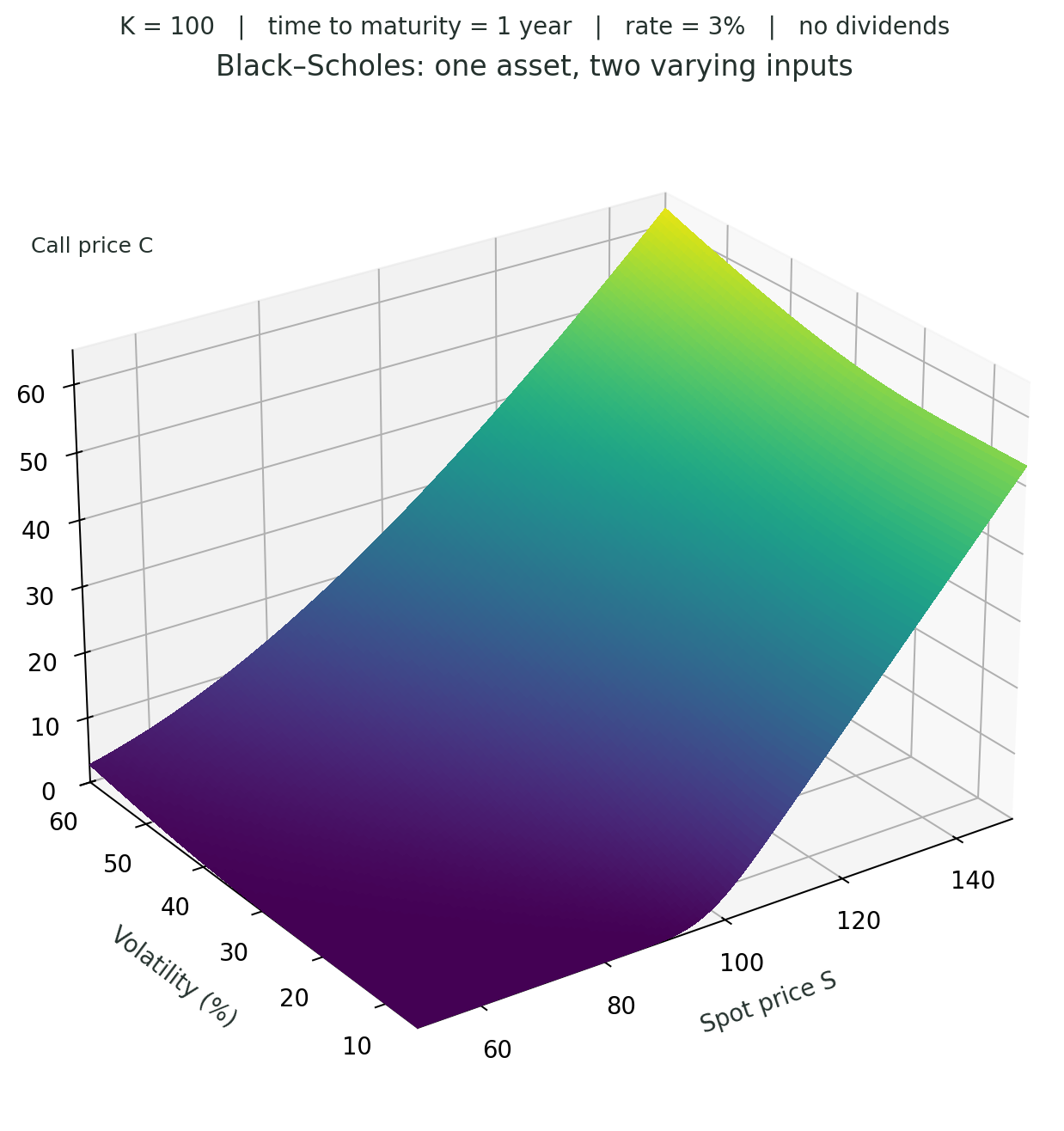
Change the stock price and volatility, and a Black–Scholes call price traces out a smooth surface. Looking at it, can you tell how much information we need to describe it?
How many components?
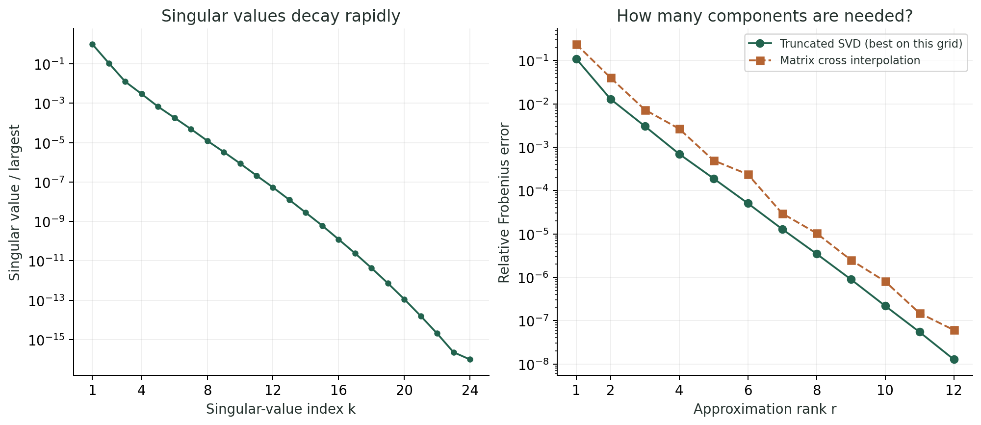
Sample the surface on a 128 × 128 grid. Low rank means approximating this table by a few products of one-variable functions:
\[ C(S,\sigma)\approx\sum_{\alpha=1}^{r}u_\alpha(S)v_\alpha(\sigma). \]The singular values fall quickly. Only a few components carry most of the information.
Rebuild the surface from a few slices
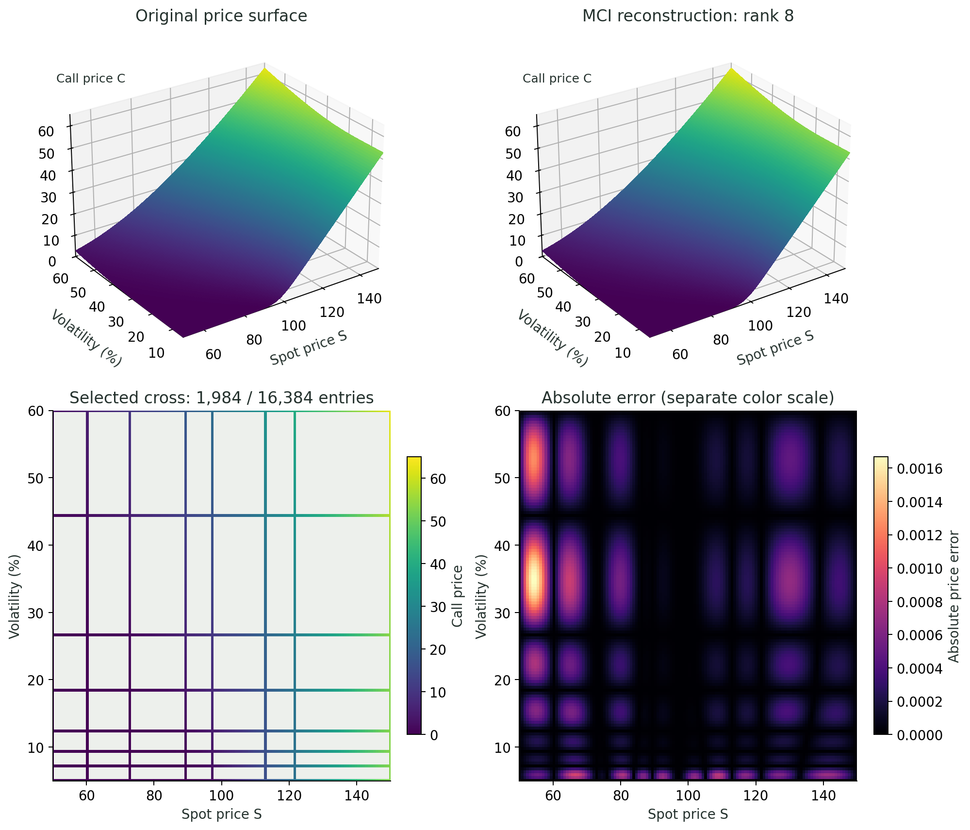
Matrix cross interpolation (MCI) combines selected rows and columns. Here, 8 rows and 8 columns reconstruct the surface with a relative error of about 0.0010%.
How much detail along each axis?
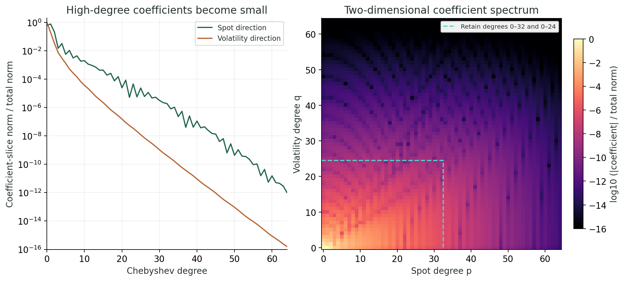
Now expand each direction in Chebyshev polynomials. Higher degrees describe finer detail. Their coefficients get small quickly, so we can drop the high-degree terms.
Low rank + low degree
Rank counts the products we add together. Degree controls the detail within each one-variable function. This example allows both to stay modest.
Keep degree 32 in stock price, degree 24 in volatility, and compress the coefficient matrix to rank 8. The result needs 464 coefficients, with relative error \(3.9\times10^{-6}\) at new test points.
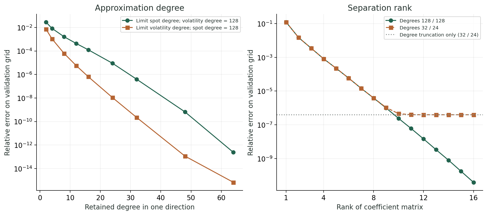
A smooth appearance is a starting point. Here, the spectra and reconstruction errors show which structure we can actually use.
Methods, accuracy, and reproducibility
The first experiment uses the Black–Scholes formula on a uniform 128 × 128 grid. All relative errors are Frobenius errors, not pointwise relative errors. The teaching MCI implementation searches the full residual: 1,984 counts retained entries, not function evaluations. Its reconstruction solves a linear system with the selected intersection matrix.
The Chebyshev experiment separately evaluates a full 129 × 129 Chebyshev–Lobatto grid. Coordinates are mapped as S = 100 + 50x and σ = 0.325 + 0.275y. A type-I discrete cosine transform gives standard, unnormalized Chebyshev coefficients through degree 128 in both directions. Coefficients are checked against a 193 × 193 construction.
Truncation to degrees 32 and 24 leaves 33 × 25 = 825 coefficients. Its relative error is 3.94 × 10⁻⁷. A separate SVD of this coefficient matrix gives rank-8 factors with 8(33 + 25) = 464 stored coefficients, including singular values absorbed into one factor. This coefficient-space SVD is not the optimal SVD for a uniform price grid.
Both polynomial errors are measured against exact prices at a disjoint 192 × 190 uniform midpoint grid. The combined degree/rank approximation has relative error 3.91 × 10⁻⁶ and maximum absolute error 5.46 × 10⁻⁴. Storage counts exclude metadata and do not describe construction costs. These are sampled checks, not bounds over the entire domain or guarantees for Greeks.
Low degree bounds the possible separation rank, but the two measures are different: a degree-32/24 coefficient matrix has rank at most 25, and here rank 8 suffices at the reported accuracy. Conversely, a product of two degree-100 polynomials can have rank 1. Results depend on the domain, model parameters, and requested accuracy.
Reproduce the figures: price surface and MCI code · Chebyshev code. Keep both scripts in the same folder. Download grid results or Chebyshev spectra, errors, and factor coefficients.
Further reading: Núñez Fernández et al., tensor cross interpolation (2025); Townsend & Trefethen, Chebfun2 (2013); SciPy’s DCT definition. For the connection to parameter-dependent option pricing: Sakurai, Takahashi & Miyamoto (2025).