Asian barrier option: a price surface
These plots evaluate a saved tensor train over moneyness \(m=S_0/K\) and volatility \(\sigma\). The degree-truncated approximation (labelled ME in the figures) retains degrees 26 and 7, with TT bond dimension 3.
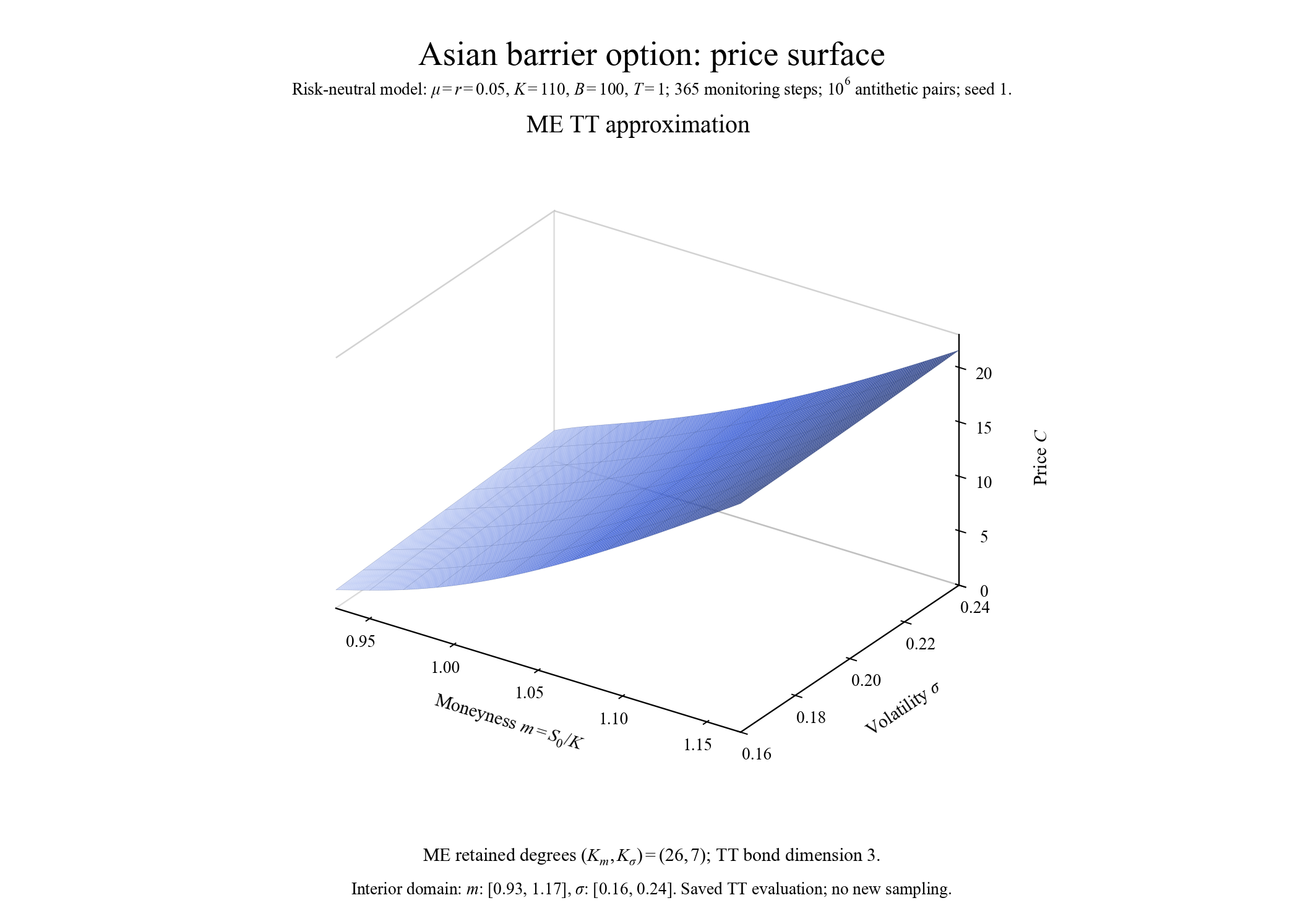
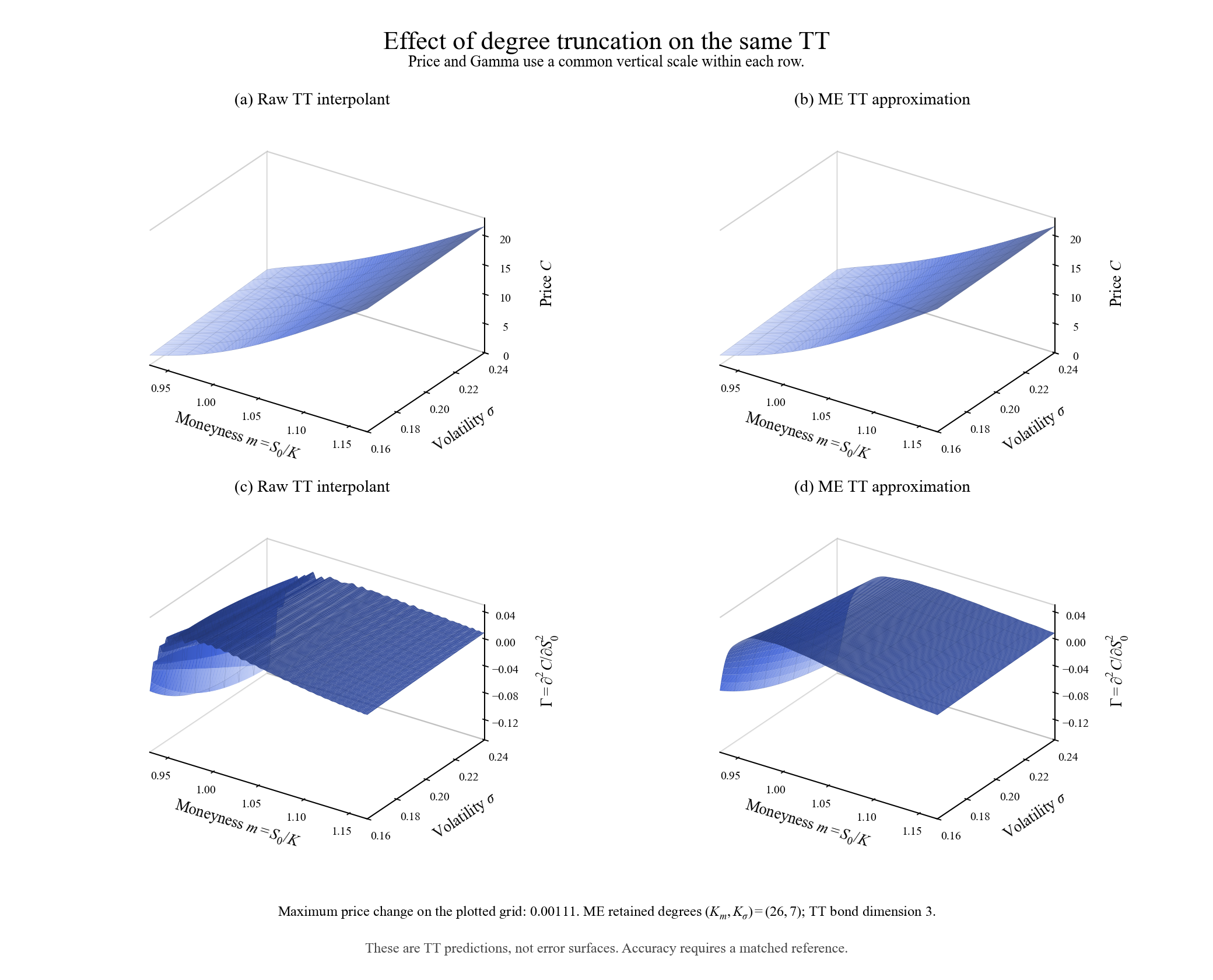
Price and Gamma
Truncation changes the price by at most 0.00111 on the plotted grid. The Gamma surface looks smoother after truncation. A matched reference is still needed to assess accuracy.
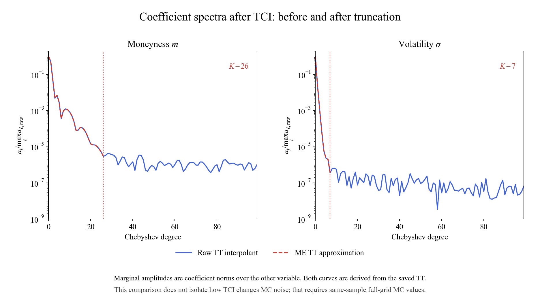
Which degrees remain?
The marginal Chebyshev coefficient amplitudes decay before reaching a small tail. The cutoffs retain degrees through 26 in moneyness and 7 in volatility.
Why so few coefficients?
What I find striking is that a calculation involving 365 path steps and a barrier can end up with such a compact representation. The paths are complicated, yet their average may have a much simpler shape.
Averaging over paths can smooth the price's dependence on its inputs. Smooth variation can make high-degree Chebyshev coefficients small. Low rank describes something else: a simple coupling between variables. Smoothness alone does not guarantee low rank. Here, the saved approximation combines modest polynomial degrees with rank 3.
When does this simplicity break down? Near the barrier, close to maturity, or over a wider parameter range? That is something I'd like to explore.
Calculation settings and source
Risk-neutral model: μ = r = 0.05, strike K = 110, barrier B = 100, maturity T = 1. There are 365 monitoring steps and 106 antithetic pairs, with seed 1.
Plotted interior domain: m ∈ [0.93, 1.17], σ ∈ [0.16, 0.24]. These are saved TT evaluations; no new sampling or reference comparison was performed for these plots.
Source: the 3 October 2026 report, Asian barrier: saved TT surfaces (final version).
Related reading: Chebyshev Interpolation for Parametric Option Pricing and Chebfun and Approximation Theory.